Kinematics & Dynamics — Theory to Simulation in ROS 2 Python with the UR Robot |《运动学与动力学 —— 从理论到 ROS 2 Python 仿真（UR 机械臂实例）》

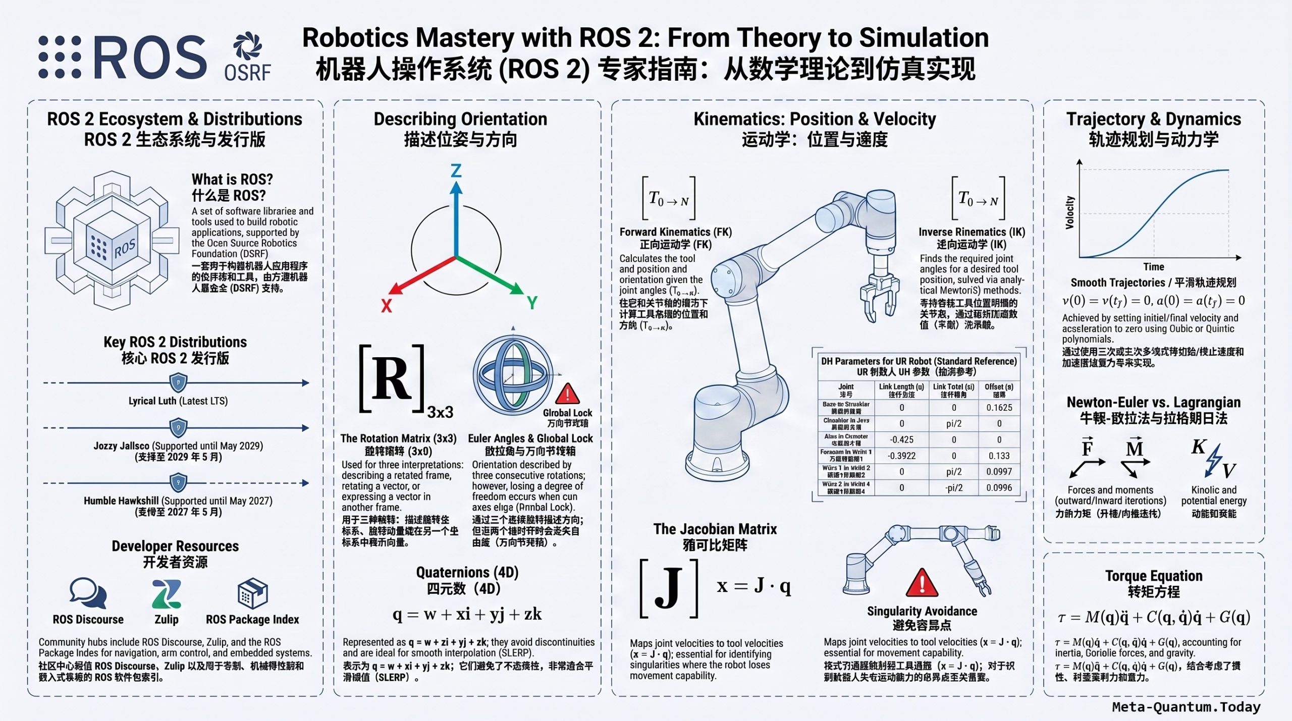
Introduction / 引言

EN — Most robotics courses stop at the whiteboard: rotation matrices, DH tables, and Jacobians derived symbolically, with little connection to how a real manipulator actually behaves. This course takes the opposite approach. Every concept — from a 2D rotation matrix to Lagrangian dynamics — is first derived on paper, then immediately verified against a live Universal Robots (UR) arm in RViz using ROS 2 and Python. The instructor screenshots the terminal output next to hand-drawn frames, checks the signs and magnitudes against the visual pose of the robot, and only moves on once theory and simulation agree. That “derive it, then prove it in RViz” loop is the throughline of the entire series, and it’s what separates this course from a typical robotics-math lecture.

The course is organized into five parts, following the natural dependency chain of manipulator kinematics: (1) Position and Orientation, (2) Kinematics, (3) Numerical Methods, (4) Trajectory Planning, and (5) Manipulator Dynamics. Each part builds directly on the last — you cannot understand DH parameters without rotation matrices, and you cannot understand the Jacobian without forward kinematics.

中文 — 大多数机器人学课程止步于黑板推导：旋转矩阵、DH 参数表、雅可比矩阵，全部停留在符号层面，很少真正连接到机械臂的实际运动。这门课程反其道而行之——从最基础的 2D 旋转矩阵到最后的拉格朗日动力学，每一个概念都先在纸面上推导，再立即用 ROS 2 + Python 在 RViz 中对真实的 Universal Robots（UR）机械臂进行验证。讲师会把终端输出的截图与手绘坐标系并排放置，逐一核对符号和数值是否与机械臂的实际姿态相符，理论与仿真吻合后才继续下一步。这种”先推导、再在 RViz 里验证”的闭环贯穿全系列，也是这门课区别于普通机器人数学课的关键之处。

课程共分五大部分，遵循机械臂运动学的自然依赖关系：（1）位置与姿态、（2）运动学、（3）数值方法、（4）轨迹规划、（5）机械臂动力学。每一部分都直接建立在前一部分之上——不理解旋转矩阵就无法理解 DH 参数，不理解正运动学就无法理解雅可比矩阵。

Video about ROS 2 | 关于 ROS 2 的视频：

Related Sections of Video | 视频相关部分

Part 1 — Position and Orientation / 第一部分：位置与姿态

EN — The course opens with the three interpretations of a rotation matrix: (1) describing a rotated frame relative to a reference frame, (2) rotating a vector by an angle, and (3) re-expressing a fixed vector in a different frame. This three-way framing is worth remembering — most confusion with rotation matrices later in a robotics career traces back to conflating these three uses. The instructor derives the 2D rotation matrix by projecting the rotated axes onto the original frame using sine and cosine, then extends it to 3D by adding an invariant axis of rotation, producing the familiar Rx, Ry, Rz matrices. Two operational properties get special emphasis because they’re used constantly downstream: rotation order matters (RxRy ≠ RyRx), and the inverse of a rotation matrix is simply its transpose — a property that makes frame-to-frame conversions computationally cheap.

From there the course moves through Euler angles (proper vs. Tait-Bryan types, and the gimbal lock problem where two joint axes align and one degree of freedom is lost), axis-angle representation (a single rotation θ about an arbitrary axis k, converted to and from a rotation matrix via Rodrigues’ formula), quaternions (four-number representation with the double-cover property q = −q, quaternion rotation via the Hamilton product, and spherical linear interpolation / SLERP for smooth orientation blending), and finally the homogeneous transformation matrix, which packages rotation and translation into a single 4×4 matrix and supports frame-chaining (T02 = T01·T12) and easy inversion via the rotation transpose.

中文 — 课程首先讲解旋转矩阵的三种解读方式：（1）描述某坐标系相对参考系旋转后的姿态；（2）将一个向量旋转某个角度；（3）把一个固定向量在另一个坐标系中重新表达。这三种视角非常值得牢记——日后在机器人工程中对旋转矩阵产生的大部分困惑，往往就是把这三种用法混淆所致。讲师先通过将旋转后的坐标轴投影到原坐标系（用正弦、余弦表示）推导出 2D 旋转矩阵，再通过增加一个不变的旋转轴将其扩展到 3D，得到熟悉的 Rx、Ry、Rz 矩阵。这里特别强调两个运算性质，因为后续会反复用到：旋转顺序会影响结果（RxRy ≠ RyRx）；旋转矩阵的逆就是其转置，这使得坐标系之间的转换在计算上非常轻量。

接下来课程讲解欧拉角（固有型 vs. Tait-Bryan 型，以及万向节死锁问题——当两个关节轴线重合时会损失一个自由度）、轴角表示法（绕任意轴 k 旋转角度 θ，通过罗德里格斯公式在旋转矩阵与轴角之间互相转换）、四元数（四维数表示，具有 q = −q 的双重覆盖性质，通过哈密顿积实现四元数旋转，并用球面线性插值 SLERP 实现姿态间的平滑过渡），最后是齐次变换矩阵——将旋转与平移打包进一个 4×4 矩阵，支持坐标系链式相乘（T02 = T01·T12）以及通过旋转部分转置实现的简便求逆。

Part 2 — Kinematics / 第二部分：运动学

EN — This is the structural core of the course. DH (Denavit-Hartenberg) parameters are introduced as the standard way to place coordinate frames on a serial-link manipulator, with a clear side-by-side comparison of the standard vs. modified conventions (differing in frame attachment order and indexing — modified DH is the one used in Craig’s textbook and throughout this course). The four DH parameters — link length a, link twist α, link offset d, and joint angle θ — are defined geometrically and then assembled into the DH transformation matrix that maps one joint frame to the next.

Forward kinematics is then just the product of all DH transformation matrices from base to tool: T0n = T01·T12·…·T(n-1)n. Inverse kinematics is treated analytically for a 2-DOF planar arm — solving for θ2 first via the law of cosines, then θ1 via atan2 — with the explicit caveat that closed-form analytical IK generally only exists for specific robot geometries (like the UR’s spherical wrist), which is the motivation for the numerical methods covered in Part 3.

中文 — 这是整门课程的结构核心。DH（Denavit-Hartenberg）参数被引入作为在串联式机械臂上放置坐标系的标准方法，课程对标准 DH 与修正 DH 两种约定进行了清晰的并列对比（区别在于坐标系附着顺序和编号方式——修正 DH 正是 Craig 教材以及本课程所采用的版本）。四个 DH 参数——连杆长度 a、连杆扭角 α、连杆偏距 d、关节角 θ ——先从几何意义上定义，再组装成描述相邻关节坐标系变换的 DH 变换矩阵。

正运动学随之变得简单：只需将从基座到末端的所有 DH 变换矩阵依次相乘，T0n = T01·T12·…·T(n-1)n。逆运动学则以一个平面 2 自由度机械臂为例采用解析法求解——先用余弦定理求 θ2，再用 atan2 求 θ1，同时明确指出：解析形式的逆运动学通常只对特定构型的机械臂成立（例如 UR 机械臂具备的球形手腕结构），这也正是第三部分引入数值方法的原因所在。

Part 3 — Numerical Methods / 第三部分：数值方法

EN — The Jacobian matrix is introduced both geometrically (mapping joint velocities to tool-tip linear and angular velocity, built column-by-column from each joint’s axis direction and position relative to the tool end) and analytically (as the partial derivative of the forward kinematics function with respect to joint angles, useful when using non-rotation-matrix orientation representations like quaternions or Euler angles). A numerical (finite-difference) version of the Jacobian is derived as a fallback when an analytical Jacobian is impractical, using forward, backward, and central difference formulas.

These two tools combine into numerical inverse kinematics via Newton’s method: iteratively minimizing a pose error vector by stepping joint angles in the direction of the pseudo-inverse Jacobian, with damped least-squares and Jacobian-transpose variants mentioned as alternatives that trade convergence speed for stability near singularities. This is presented as the general-purpose IK approach that works for any manipulator geometry, unlike the closed-form solution from Part 2.

中文 — 雅可比矩阵在本部分从两个角度引入：几何角度（将关节速度映射为末端的线速度与角速度，按每个关节的轴向以及相对末端的位置逐列构建），以及解析角度（作为正运动学函数对关节角的偏导数，当采用四元数、欧拉角等非旋转矩阵形式描述姿态时尤为有用）。当解析雅可比难以求得时，课程还给出了基于有限差分的数值雅可比，包括前向差分、后向差分与中心差分三种形式。

将这两个工具结合，便得到基于牛顿法的数值逆运动学：通过沿雅可比伪逆方向逐步迭代更新关节角，以最小化位姿误差向量；同时提到阻尼最小二乘法与雅可比转置法这两种变体，它们在奇异位形附近以收敛速度换取数值稳定性。相比第二部分的封闭解，这里给出的是适用于任意机械臂构型的通用逆运动学方法。

Part 4 — Trajectory Planning / 第四部分：轨迹规划

EN — Joint-space trajectories use cubic (and optionally quintic) polynomials to interpolate between start and end joint configurations with zero velocity (and optionally zero acceleration) at both endpoints, guaranteeing smoothness. Cartesian-space trajectories extend this idea to the tool-tip pose: linear interpolation (LERP) for position and spherical linear interpolation (SLERP) for orientation, both parameterized by the same quintic time-scaling polynomial, with the resulting pose-at-time-t converted back to joint angles at every step via inverse kinematics.

Singularity analysis follows: a manipulator loses a degree of freedom when the Jacobian’s columns become linearly dependent, which is checked via the determinant (or rank) of the Jacobian. The course demonstrates this both algebraically (fully extended or fully folded 2-DOF arm) and visually on the UR robot, where three collinear joint axes are shown producing a zero-determinant, singular Jacobian. Workspace analysis closes the section, distinguishing the reachable workspace (at least one orientation possible at each point) from the dextrous workspace (every orientation possible), and using Monte Carlo sampling over joint limits as the practical way to visualize it.

中文 — 关节空间轨迹使用三次（或五次）多项式在起始与终止关节位形之间插值，并在两端强制速度为零（五次多项式还可强制加速度为零），从而保证轨迹平滑。笛卡尔空间轨迹则将这一思路推广到末端位姿：位置采用线性插值（LERP），姿态采用球面线性插值（SLERP），二者都使用同一条五次多项式作为时间尺度函数，每个时间步得到的位姿再通过逆运动学转换回关节角。

紧接着是奇异性分析：当雅可比矩阵的列向量线性相关时，机械臂就会损失一个自由度，可以通过雅可比矩阵的行列式（或秩）来判断。课程既用代数方法演示（2 自由度机械臂完全伸展或完全折叠的情形），也在 UR 机械臂上做了可视化验证——三个关节轴共线时，雅可比矩阵行列式为零，处于奇异位形。本部分最后是工作空间分析，区分了”可达工作空间”（每一点至少存在一种可达姿态）与”灵巧工作空间”（每一点所有姿态都可达），并采用蒙特卡洛采样关节角范围的方式来实际可视化工作空间。

Part 5 — Manipulator Dynamics / 第五部分：机械臂动力学

EN — The final part covers the two classical approaches to computing joint torques: Newton-Euler (a recursive two-pass algorithm — an outward pass computing angular/linear velocities and accelerations link by link, followed by an inward pass computing forces and torques back to the base) and Lagrangian dynamics (deriving the equations of motion from kinetic and potential energy via the Euler-Lagrange equation). Both are worked through fully on a 2-DOF planar arm, arriving at the standard manipulator dynamics equation τ = M(q)q̈ + C(q,q̇)q̇ + G(q), where M is the inertia matrix, C captures Coriolis/centrifugal effects, and G is the gravity vector. The course notes a useful sanity-check technique — isolating G by setting velocities/accelerations to zero, isolating M by setting q̇=0 and perturbing q̈ column by column — and closes by running both methods live on the UR robot as it draws a circle, comparing the resulting torque plots between the two derivations.

中文 — 最后一部分讲解计算关节力矩的两种经典方法：牛顿-欧拉法（一种递归的双向算法——先做”外推”逐连杆计算角速度、线速度与加速度，再做”内推”从末端向基座反推力与力矩），以及拉格朗日动力学（通过欧拉-拉格朗日方程，从动能与势能出发推导运动方程）。两种方法都在一个 2 自由度平面机械臂上完整推导，最终得到标准的机械臂动力学方程 τ = M(q)q̈ + C(q,q̇)q̇ + G(q)，其中 M 为惯性矩阵，C 描述科氏力/离心力效应，G 为重力向量。课程还给出了实用的自检方法——令速度与加速度为零即可单独得到 G；令 q̇=0 并逐列扰动 q̈ 即可单独得到 M——最后在 UR 机械臂上实时运行两种方法，让机械臂画圆的同时对比两种推导得到的力矩曲线。

About ROS2 / 关于 ROS2

EN — Before any of the kinematics math — rotation matrices, DH parameters, Jacobians — can be verified against a real or simulated robot, you need a working ROS 2 environment. This post is the missing “step zero”: how to install ROS 2, set up a workspace, write and build your own package, and run a minimal kinematics node that publishes a computed forward-kinematics pose — the exact pattern used throughout the UR-robot kinematics course. It’s written for someone comfortable with a terminal but new to ROS 2’s conventions (workspaces, packages, nodes, topics, colcon).

中文 — 在验证任何运动学数学之前——无论是旋转矩阵、DH 参数还是雅可比矩阵——你都需要先有一个能正常运行的 ROS 2 环境。这篇文章正是缺失的”第零步”：如何安装 ROS 2、搭建工作空间、编写并编译自己的功能包，并运行一个最小化的运动学节点来发布计算出的正运动学位姿——这正是 UR 机械臂运动学课程中反复使用的模式。本文面向熟悉终端操作但尚不熟悉 ROS 2 概念（工作空间、功能包、节点、话题、colcon）的读者。

Features & Concepts / 功能与核心概念

What ROS 2 actually is / ROS 2 究竟是什么

EN — ROS 2 is not an operating system — it’s a middleware layer on top of Linux (primarily Ubuntu) that gives robotics code a standard way to communicate. The core primitives you’ll use constantly:

• Node — a single running process that does one job (e.g., “compute forward kinematics”).
• Topic — a named, typed data stream nodes publish to or subscribe from (e.g., /joint_states).
• Package — the unit of distribution: source code, build instructions, and metadata bundled together.
• Workspace — a directory tree (src/, build/, install/, log/) that holds one or more packages and gets compiled together with colcon.
• Action / Service — request-response or long-running goal-based communication, used for things like commanding a robot arm to a pose (ros2 action send_goal).

中文 — ROS 2 本身并不是一个操作系统，而是运行在 Linux（主要是 Ubuntu）之上的一层中间件，为机器人代码提供了一套标准的通信方式。以下是会反复用到的核心概念：

• 节点（Node）——一个独立运行的进程，只做一件事（例如”计算正运动学”）。
• 话题（Topic）——节点之间发布/订阅的具名、带类型的数据流（例如 /joint_states）。
• 功能包（Package）——分发的基本单元：源码、编译指令与元数据打包在一起。
• 工作空间（Workspace）——一个目录结构（src/、build/、install/、log/），容纳一个或多个功能包，并通过 colcon 统一编译。
• 动作/服务（Action / Service）——请求-响应式或基于长时间目标的通信方式，常用于命令机械臂运动到某个位姿（ros2 action send_goal）。

Setup, Configuration & a Simple Kinematics Example / 环境搭建、配置与简单实例

Step 1 — Install ROS 2 / 第一步：安装 ROS 2

EN — ROS 2 releases are distro-named (e.g., Humble, Jazzy) and each is tied to a specific Ubuntu LTS version. Check https://docs.ros.org for the release that matches your Ubuntu version before installing — this changes over time, so don’t rely on a fixed version number. The general installation pattern on Ubuntu is:

# 1. Set locale (UTF-8 required)
sudo apt update && sudo apt install -y locales
sudo locale-gen en_US en_US.UTF-8
sudo update-locale LC_ALL=en_US.UTF-8 LANG=en_US.UTF-8

# 2. Enable the ROS 2 apt repository
sudo apt install -y software-properties-common curl
sudo add-apt-repository universe
sudo curl -sSL <https://raw.githubusercontent.com/ros/rosdistro/master/ros.key> \
  -o /usr/share/keyrings/ros-archive-keyring.gpg
echo "deb [arch=$(dpkg --print-architecture) signed-by=/usr/share/keyrings/ros-archive-keyring.gpg] \
  <http://packages.ros.org/ros2/ubuntu> $(. /etc/os-release && echo $UBUNTU_CODENAME) main" \
  | sudo tee /etc/apt/sources.list.d/ros2.list > /dev/null

# 3. Install (replace <distro> with your matched ROS 2 release, e.g. jazzy)
sudo apt update
sudo apt install -y ros-<distro>-desktop

# 4. Source it in every new terminal (or add to ~/.bashrc)
source /opt/ros/<distro>/setup.bash

For Windows users following along with the UR course via WSL, install Ubuntu through WSL2 first, then run the same steps inside the WSL terminal.

中文 — ROS 2 每个发行版都有代号（如 Humble、Jazzy），并且各自对应特定的 Ubuntu LTS 版本。安装前请先到 https://docs.ros.org 确认与你 Ubuntu 版本匹配的发行版——这个对应关系会随时间变化，不要死记某个固定版本号。在 Ubuntu 上的通用安装流程如上方代码块所示：设置 UTF-8 语言环境 → 添加 ROS 2 的 apt 软件源 → 安装（将 <distro> 替换为你匹配到的版本，例如 jazzy）→ 在每个新终端中 source（或写入 ~/.bashrc）。

如果你和 UR 课程一样是在 Windows 下通过 WSL 跟着学习，先通过 WSL2 安装 Ubuntu，然后在 WSL 终端里执行同样的步骤即可。

Step 2 — Create a workspace and package / 第二步：创建工作空间与功能包

EN —

# Create the workspace source folder
mkdir -p ~/ros2_ws/src
cd ~/ros2_ws/src

# Create a Python package (this is what the UR kinematics course uses throughout)
ros2 pkg create --build-type ament_python ur_kinematics_demo \
  --dependencies rclpy geometry_msgs sensor_msgs tf2_ros

cd ~/ros2_ws
colcon build --symlink-install
source install/setup.bash

• -symlink-install means edits to your Python files take effect without rebuilding — useful while iterating on a kinematics node.

中文 —

# 创建工作空间的 src 目录
mkdir -p ~/ros2_ws/src
cd ~/ros2_ws/src

# 创建一个 Python 功能包（UR 运动学课程全程使用的正是这种类型）
ros2 pkg create --build-type ament_python ur_kinematics_demo \
  --dependencies rclpy geometry_msgs sensor_msgs tf2_ros

cd ~/ros2_ws
colcon build --symlink-install
source install/setup.bash

• -symlink-install参数的作用是：修改 Python 源文件后无需重新编译即可生效，这在调试运动学节点时非常方便。

Step 3 — Write a minimal forward-kinematics node / 第三步：编写一个最小化的正运动学节点

EN — This mirrors the pattern used throughout the UR-robot course: a node reads joint angles, computes the forward-kinematics transform via DH-parameter matrix multiplication, and publishes/prints the result. Here’s a simplified 2-DOF planar-arm version (ur_kinematics_demo/fk_node.py):

import rclpy
from rclpy.node import Node
import numpy as np

class SimpleFKNode(Node):
    def __init__(self):
        super().__init__('simple_fk_node')
        self.l1, self.l2 = 1.0, 0.8       # link lengths (m)
        self.timer = self.create_timer(1.0, self.compute_fk)

    def compute_fk(self):
        theta1, theta2 = np.pi / 4, np.pi / 6  # example joint angles (rad)

        def dh_transform(theta, d, a, alpha):
            ct, st = np.cos(theta), np.sin(theta)
            ca, sa = np.cos(alpha), np.sin(alpha)
            return np.array([
                [ct, -st * ca,  st * sa, a * ct],
                [st,  ct * ca, -ct * sa, a * st],
                [0,        sa,       ca,      d],
                [0,         0,        0,      1]
            ])

        T01 = dh_transform(theta1, 0, self.l1, 0)
        T12 = dh_transform(theta2, 0, self.l2, 0)
        T02 = T01 @ T12

        pos = T02[:3, 3]
        self.get_logger().info(f'Tool-end position: x={pos[0]:.3f}, y={pos[1]:.3f}, z={pos[2]:.3f}')

def main():
    rclpy.init()
    node = SimpleFKNode()
    rclpy.spin(node)
    node.destroy_node()
    rclpy.shutdown()

if __name__ == '__main__':
    main()

Register it as an entry point in setup.py:

entry_points={
    'console_scripts': [
        'fk_node = ur_kinematics_demo.fk_node:main',
    ],
},

中文 — 这个例子沿用了 UR 机械臂课程中贯穿始终的模式：节点读取关节角，通过 DH 参数矩阵相乘计算正运动学变换，再发布/打印结果。以下是一个简化版的 2 自由度平面机械臂示例（ur_kinematics_demo/fk_node.py，代码见上方代码块）。

需要在 setup.py 中注册对应的入口点（同样见上方代码块），这样才能通过 ros2 run 调用该节点。

Step 4 — Build, run, and verify / 第四步：编译、运行与验证

EN —

cd ~/ros2_ws
colcon build --symlink-install
source install/setup.bash
ros2 run ur_kinematics_demo fk_node

Expected output, printed once per second:

[INFO] [simple_fk_node]: Tool-end position: x=1.190, y=1.269, z=0.000

To sanity-check it the same way the course does — visually — you’d add a static/robot-state publisher and view the frame in RViz (rviz2), or compare the printed x/y against a hand sketch of the two-link arm at θ1=45°, θ2=30°. To inspect the live data stream instead of the log line, publish the pose on a topic and check it with:

ros2 topic list
ros2 topic echo /tool_end_pose

中文 —

编译、source、运行三步如上方代码块所示。预期每秒打印一次输出，例如：

[INFO] [simple_fk_node]: Tool-end position: x=1.190, y=1.269, z=0.000

要像课程中那样做”可视化自检”，可以添加一个静态/机器人状态发布器，并在 RViz（rviz2）中查看对应坐标系；或者直接用 θ1=45°、θ2=30° 手绘一个双连杆机械臂草图，与打印出的 x/y 数值核对。如果想查看实时数据流而不是日志输出，可以将位姿发布到一个话题上，再用以下命令查看：

ros2 topic list
ros2 topic echo /tool_end_pose

Common configuration pitfalls / 常见配置陷阱

EN —

• The course’s defining strength is its derive-then-verify loop: every mathematical result is checked against a physical (simulated) UR robot’s actual pose in RViz, closing the gap between symbolic math and physical intuition that most robotics courses leave open.
• The five-part structure mirrors the real dependency chain of manipulator kinematics — orientation representations → kinematics (DH, FK, analytical IK) → numerical methods (Jacobian, numerical IK) → trajectory planning → dynamics — making it a coherent curriculum rather than a loose collection of topics.
• Two properties worth remembering independent of the rest: rotation order always matters, and a rotation matrix’s inverse is its transpose — both save real debugging time when working with TF trees in ROS.
• Analytical IK is elegant but geometry-specific; numerical (Jacobian-based) IK is the generalizable tool that works on arbitrary manipulators, which is why the course deliberately teaches both.
• For engineers already working with PLC/industrial control systems or Odoo-style automation stacks, the DH-parameter-to-transformation-matrix pipeline and the Newton-Euler torque derivation are the most directly transferable pieces — they’re exactly what’s needed for actuator sizing or motion-control tuning on a real serial-link arm.
• Mismatched ROS 2 distro vs. Ubuntu version — always cross-check on docs.ros.org rather than assuming.

中文 —

• 本课程最鲜明的特色在于**”推导—验证”闭环**：每一个数学结果都会与仿真中真实 UR 机械臂在 RViz 里呈现的姿态进行比对，弥合了大多数机器人课程留下的”符号数学”与”物理直觉”之间的鸿沟。
• 五大部分的结构完整反映了机械臂运动学的真实依赖链条——姿态表示 → 运动学（DH、正运动学、解析逆运动学）→ 数值方法（雅可比矩阵、数值逆运动学）→ 轨迹规划 → 动力学——因此这是一套连贯的课程体系，而非零散主题的堆砌。
• 有两点即便脱离具体课程内容也值得牢记：旋转顺序始终会影响结果；旋转矩阵的逆就是其转置——这两点在处理 ROS 的 TF 坐标树时能实实在在节省调试时间。
• 解析法逆运动学优雅但依赖特定几何构型；数值法（基于雅可比）逆运动学则是可推广到任意机械臂构型的通用工具，这正是课程刻意讲授两者的原因。
• 对于已经在从事 PLC/工业控制系统或 Odoo 类自动化技术栈的工程师而言，”DH 参数 → 变换矩阵”这条流水线，以及牛顿-欧拉力矩推导，是最能直接迁移到实际工作中的部分——它们正是在真实串联机械臂上进行执行器选型或运动控制调参所需要的知识。
• ROS 2 发行版与 Ubuntu 版本不匹配——务必到 docs.ros.org 核实，而不是凭经验假设。

Conclusion & Key Takeaways / 结论与要点总结

EN —

• ROS 2’s core mental model is small: nodes talk over topics/services/actions, packages bundle code, workspaces bundle packages, and colcon builds everything together.
• The install-locale-repo-package sequence is standard across ROS 2 releases; only the distro codename changes, so always confirm it against your Ubuntu version at docs.ros.org rather than copying an old tutorial’s exact version string.
• A kinematics node is just a normal ROS 2 node that happens to do matrix math (here, DH-parameter transforms) and publish or log the result — the same pattern scales from a 2-DOF toy arm to a 6-DOF UR robot.
• -symlink-install and rosdep install are the two habits that save the most iteration time when developing kinematics nodes.

中文 —

• ROS 2 的核心心智模型很简单：节点通过话题/服务/动作互相通信，功能包打包代码，工作空间打包功能包，colcon 统一编译一切。
• “设置语言环境 → 添加软件源 → 安装功能包”这一流程在各个 ROS 2 发行版之间是通用的，唯一会变的是发行版代号，所以务必到 docs.ros.org 根据自己的 Ubuntu 版本确认，而不要照搬旧教程里的固定版本号。
• 所谓”运动学节点”，本质上就是一个普通的 ROS 2 节点，只不过做的是矩阵运算（这里是 DH 参数变换），并把结果发布或打印出来——这套模式从 2 自由度的玩具机械臂到 6 自由度的 UR 机械臂都同样适用。
• -symlink-install 与 rosdep install 是开发运动学节点时最能节省调试时间的两个习惯。

References / 参考资料

• ROS 2 official documentation (installation, distro compatibility) — https://docs.ros.org
• colcon build tool documentation — https://colcon.readthedocs.io
• Denavit–Hartenberg parameters (general reference) — https://en.wikipedia.org/wiki/Denavit–Hartenberg_parameters
• Spong, M. W. & Vidyasagar, M., Robot Dynamics and Control, John Wiley & Sons — standard reference for the Newton-Euler and Lagrangian formulations covered in Part 5.
• Craig, J. J., Introduction to Robotics: Mechanics and Control — the textbook source for the modified DH convention used throughout this course.